GTFermiSurfaceCut
GTFermiSurfaceCut[Hamiltonian,Fermi energy,list of bands,ndel,plane, area] calculates a cut throught the Fermi surface corresponding to a Hamiltonian and Fermi energy if the Fermi surface contains parts from list of bands. The electronic structure is calculated in a cube at ndel points per spatial dimension. plane defines orientation and position of the cutting plane. area defines a quadratic region in the cutting plane.
Examplesopen all
Basic Examples (1)
| In[1]:= |
| In[2]:= |
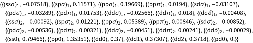
Read the TB parameterset for Cu.
Read the predefined ![]() Hamiltonian for the fcc structure.
Hamiltonian for the fcc structure.
| In[4]:= |
The Hamiltonian for Cu is prepared by insertion of the parameter set.
| In[5]:= |
To see that all works correctly, the band structure is calculated. This is not necessary for the construction of the XCrySDen files.


The exact position of the Fermi energy can be found from the DOS. We calculate the isoenergetic surface to E = 0.6 Ryd for band number 6


Now we create a cut throught the Fermi surface. We want to see the cut in the kk-ky-plane. Thus the normal vector will be (0,0,1) amd the shift vector (0,0,0).
| In[8]:= |
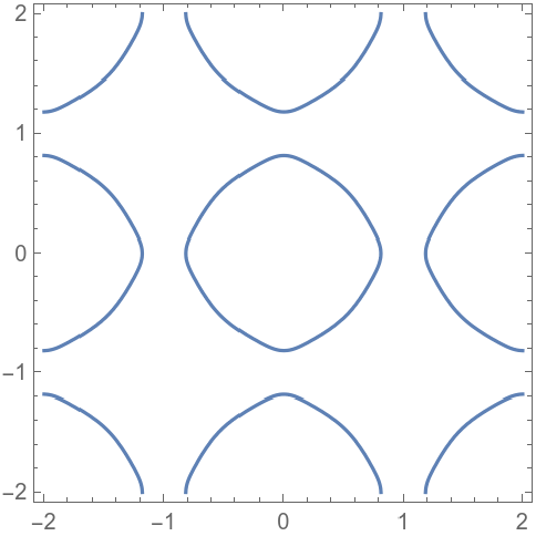
The Brillouin zone boundaries in this plane can be added to the plot.
| In[10]:= |

| In[11]:= |

